Deffuant et al.'s Bounded Confidence Model of Opinion Dynamics
Source:vignettes/boundedconfidence.Rmd
boundedconfidence.RmdRead about the Bounded Confidence Model of Opinion Dynamics in the original publication of 2000 by Deffuant, Neau, Amblard, and Weisbuch.
The version implemented here sets up 100 agents and distributes an opinion, operationalized on a normalized scale with an average (mean) of 0 and a standard deviation of 1, thus roughly ranging from -2 to +2. In each round, each agent meets with a random other agent whereby both update their opinion according to a slightly varying adaptation factor my (a random number between a lower and an upper boundary of my) if, any only if, their opinion delta is below a certain threshold.
library(tidyabm)
library(dplyr)
#>
#> Attaching package: 'dplyr'
#> The following objects are masked from 'package:stats':
#>
#>     filter, lag
#> The following objects are masked from 'package:base':
#>
#>     intersect, setdiff, setequal, union
library(ggplot2)
Model configuration parameters are combined here:
n_agents <- 100
threshold <- 2.0
my_lower_boundary <- 0.0
my_upper_boundary <- 0.5
This time, creating the agent blueprints is kind of useless. That’s because we do not give agents neither an individual opinion nor an action. We do not give them an opinion because we want to give all agents together a distribution of opinions so that the initial opinions are distributed normally. We also do not give the agents their own actions because, if specified on a per-agent level, each agent would look for another one and, hence, some would end up being in multiple meetings (because they reached out to one other agent and were reached out to by one or several other agents as well).
So instead of specifying agent blueprints, here’s the actual model (i.e., the environment) directly. Here, we add “empty” agents, distribute the initial opinions, and specify the meeting action between two random agents.
The most complicated part here are of course the meetings. For the meetings, specifically, we do the following (once per iteration/tick):
- we create
n_agents/2meetings and put them into a vector ofn_agentselements so that each meeting appears twice in this list - we distribute all agents onto these meetings so that each agent is on exactly one meeting
- for each meeting …
- we calculate the delta between the two agents’ opinions
- if the delta is larger than
thresholdwe omit this meeting - otherwise, we take a random my (between the specified lower/upper boundary) and calculate both agents’ new opinion
- finally, we iterate through the meeting results (using a quicker
iteration function named
mapout of tidyverse’s purrr package) and overwrite all the agents’ old opinions with their new opinions (note that, insidemapwe need to overwrite anything that is outside such asmewith a double arrow<<-)
For overall environment/model interpretation, we calculate pull out
the highest and lowest opinion per tick for later inspection. Also note
that the environment does not get an end point but will run
indefinitely. Hence, you have to set the max_iterations in
the iterate(...) function accordingly to when you want it
to stop:
e <- create_network_environment(seed = 13485) %>%
  add_agents(create_agent(),
             n = n_agents) %>%
  distribute_characteristic_across_agents('opinion',
                                          rnorm(n = n_agents,
                                                mean = 0,
                                                sd = 1)) %>%
  add_rule('random agent meetings',
           .consequence = function(me, abm) {
             meetings <- sample(rep(1:(n_agents/2), 2))
             meeting_results <- me %>%
               convert_agents_to_tibble() %>%
               bind_cols(tibble(meeting = meetings)) %>%
               select(meeting, .id, opinion) %>%
               group_by(meeting) %>%
               summarize(agent_1 = first(.id),
                         agent_2 = last(.id),
                         opinion_1 = first(opinion),
                         opinion_2 = last(opinion),
                         .groups = 'drop') %>%
               mutate(delta = abs(opinion_1 - opinion_2)) %>%
               filter(delta <= threshold) %>%
               mutate(my = runif(n(),
                                 min = my_lower_boundary,
                                 max = my_upper_boundary),
                      opinion_new_1 = opinion_1 + my * (opinion_2 - opinion_1),
                      opinion_new_2 = opinion_2 + my * (opinion_1 - opinion_2))
             purrr::map(1:nrow(meeting_results),
                        function(meeting) {
                          me <<- me %>%
                            distribute_characteristic_across_agents(
                              'opinion',
                              meeting_results[[meeting, 'opinion_new_1']],
                              .id == meeting_results[[meeting, 'agent_1']],
                              .overwrite = TRUE,
                              .suppress_warnings = TRUE) %>%
                            distribute_characteristic_across_agents(
                              'opinion',
                              meeting_results[[meeting, 'opinion_new_2']],
                              .id == meeting_results[[meeting, 'agent_2']],
                              .overwrite = TRUE,
                              .suppress_warnings = TRUE)
                        })
             return(me)
           }) %>%
  add_variable(min_opinion = function(me, abm) {
    abm %>%
      convert_agents_to_tibble() %>%
      summarise(minimum = min(opinion)) %>%
      pull(minimum) %>%
      return()
  }) %>%
  add_variable(max_opinion = function(me, abm) {
    abm %>%
      convert_agents_to_tibble() %>%
      summarise(maximum = max(opinion)) %>%
      pull(maximum) %>%
      return()
  }) %>%
  init()
Finally, iteration. This is the step that takes a while. Note that we set a maximum of 20 iterations here so the iteration ticks exactly 20 times (because there is no other way for it to stop):
e <- e %>%
  iterate(max_iterations = 20)
#> [1] "Tick 1 finished in 3.279 secs:"
#> [1] "  min_opinion: -2.78512566739624"
#> [1] "  max_opinion: 2.62032851479196"
#> [1] "Tick 2 finished in 3.39 secs:"
#> [1] "  min_opinion: -2.51746077728397"
#> [1] "  max_opinion: 2.62032851479196"
#> [1] "Tick 3 finished in 3.418 secs:"
#> [1] "  min_opinion: -2.37934428861777"
#> [1] "  max_opinion: 2.01669245352312"
#> [1] "Tick 4 finished in 3.316 secs:"
#> [1] "  min_opinion: -1.55958351868582"
#> [1] "  max_opinion: 2.01669245352312"
#> [1] "Tick 5 finished in 3.432 secs:"
#> [1] "  min_opinion: -1.55958351868582"
#> [1] "  max_opinion: 2.01669245352312"
#> [1] "Tick 6 finished in 3.528 secs:"
#> [1] "  min_opinion: -1.41499639308866"
#> [1] "  max_opinion: 1.89535509730667"
#> [1] "Tick 7 finished in 3.604 secs:"
#> [1] "  min_opinion: -1.30345679299076"
#> [1] "  max_opinion: 1.41591201735925"
#> [1] "Tick 8 finished in 3.607 secs:"
#> [1] "  min_opinion: -1.09726134291104"
#> [1] "  max_opinion: 0.894593571568961"
#> [1] "Tick 9 finished in 3.726 secs:"
#> [1] "  min_opinion: -0.930620809004355"
#> [1] "  max_opinion: 0.691073318067747"
#> [1] "Tick 10 finished in 3.698 secs:"
#> [1] "  min_opinion: -0.772261421122725"
#> [1] "  max_opinion: 0.671915088728044"
#> [1] "Tick 11 finished in 3.597 secs:"
#> [1] "  min_opinion: -0.668620608977825"
#> [1] "  max_opinion: 0.584869739320502"
#> [1] "Tick 12 finished in 3.624 secs:"
#> [1] "  min_opinion: -0.553719457872648"
#> [1] "  max_opinion: 0.400198399768659"
#> [1] "Tick 13 finished in 3.709 secs:"
#> [1] "  min_opinion: -0.542052598604424"
#> [1] "  max_opinion: 0.367722105806354"
#> [1] "Tick 14 finished in 3.696 secs:"
#> [1] "  min_opinion: -0.437728305717494"
#> [1] "  max_opinion: 0.364408484791451"
#> [1] "Tick 15 finished in 3.782 secs:"
#> [1] "  min_opinion: -0.309114193130515"
#> [1] "  max_opinion: 0.280808473087339"
#> [1] "Tick 16 finished in 3.596 secs:"
#> [1] "  min_opinion: -0.295983040655522"
#> [1] "  max_opinion: 0.261930793025223"
#> [1] "Tick 17 finished in 3.623 secs:"
#> [1] "  min_opinion: -0.108181681069579"
#> [1] "  max_opinion: 0.224279487997386"
#> [1] "Tick 18 finished in 3.668 secs:"
#> [1] "  min_opinion: -0.0764829158714187"
#> [1] "  max_opinion: 0.190605910749892"
#> [1] "Tick 19 finished in 3.613 secs:"
#> [1] "  min_opinion: -0.042233187948907"
#> [1] "  max_opinion: 0.180475814086634"
#> [1] "Tick 20 finished in 3.649 secs:"
#> [1] "  min_opinion: 0.00886191691704735"
#> [1] "  max_opinion: 0.16375595929756"
Let’s look at the environment and also some of the agents.
e
#> # A tibble: 20 × 6
#>    .tick min_opinion max_opinion .runtime      .n_agents_after_tick
#>  * <dbl>       <dbl>       <dbl> <drtn>                       <int>
#>  1     1    -2.79          2.62  3.279230 secs                  100
#>  2     2    -2.52          2.62  3.390262 secs                  100
#>  3     3    -2.38          2.02  3.418460 secs                  100
#>  4     4    -1.56          2.02  3.316467 secs                  100
#>  5     5    -1.56          2.02  3.431823 secs                  100
#>  6     6    -1.41          1.90  3.527779 secs                  100
#>  7     7    -1.30          1.42  3.604338 secs                  100
#>  8     8    -1.10          0.895 3.607182 secs                  100
#>  9     9    -0.931         0.691 3.726223 secs                  100
#> 10    10    -0.772         0.672 3.697558 secs                  100
#> 11    11    -0.669         0.585 3.596982 secs                  100
#> 12    12    -0.554         0.400 3.624002 secs                  100
#> 13    13    -0.542         0.368 3.708517 secs                  100
#> 14    14    -0.438         0.364 3.695828 secs                  100
#> 15    15    -0.309         0.281 3.781880 secs                  100
#> 16    16    -0.296         0.262 3.596024 secs                  100
#> 17    17    -0.108         0.224 3.622561 secs                  100
#> 18    18    -0.0765        0.191 3.668239 secs                  100
#> 19    19    -0.0422        0.180 3.613080 secs                  100
#> 20    20     0.00886       0.164 3.649438 secs                  100
#> # ℹ 1 more variable: .finished_after_tick <lgl>
#> # ABM network environment
#> * undirected, 100 agents
#> * 0 environment characteristic(s),
#> * 2 environment variable(s),
#> * 1 environment rule(s),
#> * simulating (20 tick(s) passed)

e %>%
  convert_agents_to_tibble()
#> # A tibble: 100 × 4
#>    .id   .indegree .outdegree opinion
#>    <chr> <list>    <list>       <dbl>
#>  1 A1    <NULL>    <NULL>      0.143
#>  2 A2    <NULL>    <NULL>      0.0546
#>  3 A3    <NULL>    <NULL>      0.0523
#>  4 A4    <NULL>    <NULL>      0.141
#>  5 A5    <NULL>    <NULL>      0.142
#>  6 A6    <NULL>    <NULL>      0.0697
#>  7 A7    <NULL>    <NULL>      0.0460
#>  8 A8    <NULL>    <NULL>      0.0145
#>  9 A9    <NULL>    <NULL>      0.0835
#> 10 A10   <NULL>    <NULL>      0.0957
#> # ℹ 90 more rows
Finally, let’s see how the distribution of opinions has adjusted (converged) over time. We look at the mean, minimum and maximum opinion in each tick and visualize it over time. You can see the starting point that is quite (as in: normally distributed) scattered and the subsequent homogenization of opinions.
e %>%
  ggplot(aes(x = .tick,
             ymin = min_opinion,
             ymax = max_opinion)) +
  geom_linerange() +
  scale_x_continuous('Time [ticks]') +
  scale_y_continuous('Distribution of Opinions [M with min/max]') +
  theme_minimal() +
  ggtitle('Opinion Dynamics over Time')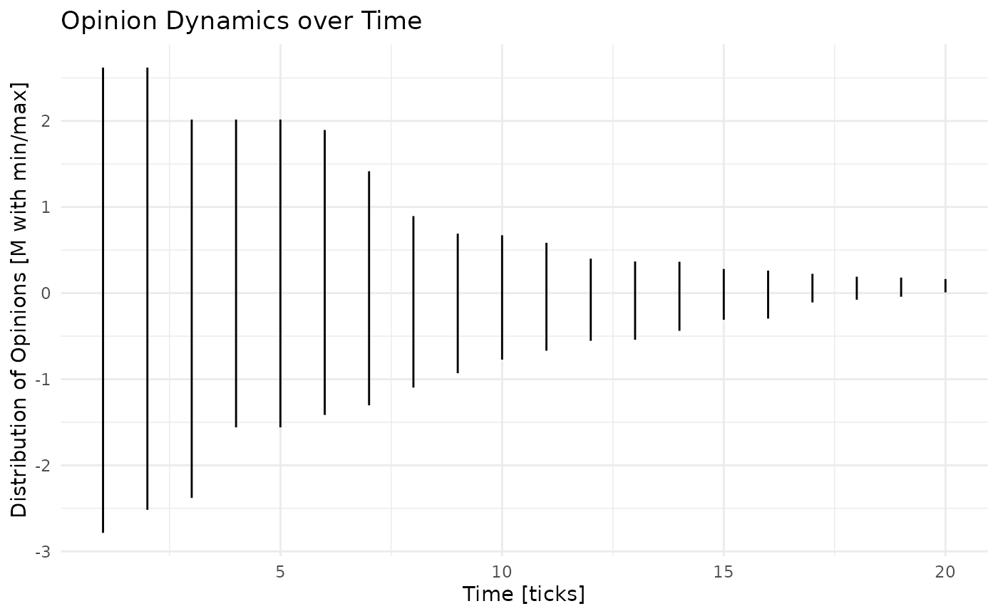
There is an alternative way, though. One where we iterate tick by
tick to collect each agent’s opinion at every point in time. This also
allows us to follow one particular agent over time in its dynamics of
opinion formation. For that, we start over with the modeling environment
(reset and init, again, and also resetting the
opinions to starting values) and then loop through 20 steps in each of
which we only tick the environment once and extract all agents’
information. The agent information we append (bind_rows) to
a variable/tibble that gets built with three columns, one identifying
the agent, one identifying the tick, and one with the opinion of that
agent after that tick. Finally, we can look at the tibble and, of
course, visualize it (whereby we also color one of the agents,
A100, blue, and all the others lightly red).
e <- e %>%
  reset() %>%
  distribute_characteristic_across_agents('opinion',
                                          rnorm(n = n_agents,
                                                mean = 0,
                                                sd = 1),
                                          .overwrite = TRUE,
                                          .suppress_warnings = TRUE) %>%
  init()

agent_opinions_over_time <- NULL

for (i in 1:20) {
  e <- e %>%
    tick()
  agent_opinions_over_time <- agent_opinions_over_time %>%
    bind_rows(e %>%
                convert_agents_to_tibble() %>%
                mutate(tick = i) %>%
                select(agent = .id,
                       tick,
                       opinion))
}
#> [1] "Tick 1 finished in 0.069 secs:"
#> [1] "  min_opinion: -2.30542578505797"
#> [1] "  max_opinion: 2.49858719659045"
#> [1] "Tick 2 finished in 3.18 secs:"
#> [1] "  min_opinion: -2.30542578505797"
#> [1] "  max_opinion: 2.49858719659045"
#> [1] "Tick 3 finished in 3.381 secs:"
#> [1] "  min_opinion: -2.30542578505797"
#> [1] "  max_opinion: 2.49858719659045"
#> [1] "Tick 4 finished in 3.249 secs:"
#> [1] "  min_opinion: -2.21144998932492"
#> [1] "  max_opinion: 2.49858719659045"
#> [1] "Tick 5 finished in 3.355 secs:"
#> [1] "  min_opinion: -2.21144998932492"
#> [1] "  max_opinion: 2.49858719659045"
#> [1] "Tick 6 finished in 3.338 secs:"
#> [1] "  min_opinion: -2.21144998932492"
#> [1] "  max_opinion: 2.49858719659045"
#> [1] "Tick 7 finished in 3.421 secs:"
#> [1] "  min_opinion: -2.21144998932492"
#> [1] "  max_opinion: 2.49858719659045"
#> [1] "Tick 8 finished in 3.289 secs:"
#> [1] "  min_opinion: -2.21144998932492"
#> [1] "  max_opinion: 2.49858719659045"
#> [1] "Tick 9 finished in 3.371 secs:"
#> [1] "  min_opinion: -2.21144998932492"
#> [1] "  max_opinion: 2.49858719659045"
#> [1] "Tick 10 finished in 3.408 secs:"
#> [1] "  min_opinion: -2.21144998932492"
#> [1] "  max_opinion: 2.49858719659045"
#> [1] "Tick 11 finished in 3.503 secs:"
#> [1] "  min_opinion: -2.21144998932492"
#> [1] "  max_opinion: 2.49858719659045"
#> [1] "Tick 12 finished in 3.532 secs:"
#> [1] "  min_opinion: -1.94932818719582"
#> [1] "  max_opinion: 2.49858719659045"
#> [1] "Tick 13 finished in 3.384 secs:"
#> [1] "  min_opinion: -1.12452784634629"
#> [1] "  max_opinion: 2.49858719659045"
#> [1] "Tick 14 finished in 3.419 secs:"
#> [1] "  min_opinion: -0.900451639436226"
#> [1] "  max_opinion: 2.49858719659045"
#> [1] "Tick 15 finished in 3.526 secs:"
#> [1] "  min_opinion: -0.816468341548787"
#> [1] "  max_opinion: 2.49858719659045"
#> [1] "Tick 16 finished in 3.499 secs:"
#> [1] "  min_opinion: -0.700740831736342"
#> [1] "  max_opinion: 2.49858719659045"
#> [1] "Tick 17 finished in 3.559 secs:"
#> [1] "  min_opinion: -0.439367597300792"
#> [1] "  max_opinion: 2.49858719659045"
#> [1] "Tick 18 finished in 3.465 secs:"
#> [1] "  min_opinion: -0.371866704707868"
#> [1] "  max_opinion: 2.49858719659045"
#> [1] "Tick 19 finished in 3.47 secs:"
#> [1] "  min_opinion: -0.323934237385286"
#> [1] "  max_opinion: 2.49858719659045"
#> [1] "Tick 20 finished in 3.474 secs:"
#> [1] "  min_opinion: -0.315911069402969"
#> [1] "  max_opinion: 2.49858719659045"

# this is the environment after being ticked 20 times
e
#> # A tibble: 20 × 6
#>    .tick min_opinion max_opinion .runtime        .n_agents_after_tick
#>  * <dbl>       <dbl>       <dbl> <drtn>                         <int>
#>  1     1      -2.31         2.50 0.06904984 secs                  100
#>  2     2      -2.31         2.50 3.17970324 secs                  100
#>  3     3      -2.31         2.50 3.38149714 secs                  100
#>  4     4      -2.21         2.50 3.24921250 secs                  100
#>  5     5      -2.21         2.50 3.35498118 secs                  100
#>  6     6      -2.21         2.50 3.33772993 secs                  100
#>  7     7      -2.21         2.50 3.42126584 secs                  100
#>  8     8      -2.21         2.50 3.28851414 secs                  100
#>  9     9      -2.21         2.50 3.37132764 secs                  100
#> 10    10      -2.21         2.50 3.40830517 secs                  100
#> 11    11      -2.21         2.50 3.50273871 secs                  100
#> 12    12      -1.95         2.50 3.53168201 secs                  100
#> 13    13      -1.12         2.50 3.38401628 secs                  100
#> 14    14      -0.900        2.50 3.41868591 secs                  100
#> 15    15      -0.816        2.50 3.52599406 secs                  100
#> 16    16      -0.701        2.50 3.49918771 secs                  100
#> 17    17      -0.439        2.50 3.55872226 secs                  100
#> 18    18      -0.372        2.50 3.46546888 secs                  100
#> 19    19      -0.324        2.50 3.46992302 secs                  100
#> 20    20      -0.316        2.50 3.47420835 secs                  100
#> # ℹ 1 more variable: .finished_after_tick <lgl>
#> # ABM network environment
#> * undirected, 100 agents
#> * 0 environment characteristic(s),
#> * 2 environment variable(s),
#> * 1 environment rule(s),
#> * simulating (20 tick(s) passed)

# this is our collected variable/tibble
agent_opinions_over_time
#> # A tibble: 2,000 × 3
#>    agent  tick opinion
#>    <chr> <int>   <dbl>
#>  1 A1        1  0.224
#>  2 A2        1  1.18
#>  3 A3        1  0.682
#>  4 A4        1  0.435
#>  5 A5        1 -0.0864
#>  6 A6        1  0.690
#>  7 A7        1 -0.440
#>  8 A8        1 -1.37
#>  9 A9        1 -0.189
#> 10 A10       1  0.692
#> # ℹ 1,990 more rows

# and this is the visualization
agent_opinions_over_time %>%
  ggplot(aes(x = tick,
             y = opinion,
             color = agent == 'A100',
             alpha = ifelse(agent == 'A100', 1, 1/10),
             group = agent)) +
  geom_point() +
  geom_line() +
  scale_x_continuous('Time [ticks]') +
  scale_y_continuous('Opinion') +
  scale_color_brewer(palette = 'Set1') +
  theme_minimal() +
  theme(legend.position = 'none') +
  ggtitle('Opinion Dynamics per Agent over Time')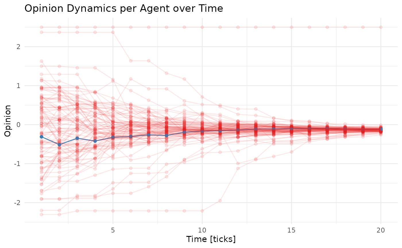
As always, we can compile relevant data for any publication we’re preparing through the ODD protocol:
e %>%
  odd()
#> # A tibble: 7 × 4
#>   `ODD category`  Element                          Content `tidyABM information`
#>   <chr>           <chr>                            <chr>   <chr>
#> 1 Overview        Purpose and patterns             "Brief… NA
#> 2 Overview        Entities, state variables, and … "List … ABM network environm…
#> 3 Overview        Process overview and scheduling  "Provi… environment rules: r…
#> 4 Design concepts Design concepts                  "This … Model has not yet fi…
#> 5 Details         Initialization                   "Speci… See the list of agen…
#> 6 Details         Input data                       "Repor… NA
#> 7 Details         Submodels                        "Repea… NA