Read about Schelling’s Segregation model in the original publication of 1971 or on Wikipedia.
The version implemented here sets up a squared grid of 20 by 20 spots. Neighborhood is defined as the surrounding up-to 8 fields of a particular agent.
library(tidyabm)
library(dplyr)
#>
#> Attaching package: 'dplyr'
#> The following objects are masked from 'package:stats':
#>
#>     filter, lag
#> The following objects are masked from 'package:base':
#>
#>     intersect, setdiff, setequal, union
library(ggplot2)
Model configuration parameters are combined here:
grid_side_length <- 20
density <- .70
neighborhood_definition <- 'o'
unhappy_similarity_threshold <- .15
Let’s create the agents (or, their blueprints):
agent_a <- create_agent() %>%
  set_characteristic(color = 'red') %>%
  add_variable(similar = function(me, abm) {
    neighbors <- grid_get_neighbors(me,
                                    abm,
                                    which = neighborhood_definition)
    n_neighbors <- nrow(neighbors)
    if (n_neighbors == 0) {
      return(0.0)
    } else {
      return(sum(neighbors$color == me$color)/n_neighbors)
    }
  }) %>%
  add_variable(unhappy = function(me, abm) {
    return(me$similar < unhappy_similarity_threshold)
  }) %>%
  add_rule('move',
           unhappy == TRUE,
           .consequence = function(me, abm) {
             spot <- grid_get_free_spots(abm) %>%
               slice_sample(n = 1)
             grid_move(me,
                       abm,
                       new_x = spot$x,
                       new_y = spot$y) %>%
               return()
           })

agent_b <- agent_a %>%
  set_characteristic(color = 'blue',
                     .overwrite = TRUE)
#> Warning: The following characteristics already existed. They were overwritten:
#> color
Here’s the actual model (i.e., the environment):
e <- create_grid_environment(seed = 38468,
                             size = grid_side_length) %>%
  add_agents(agent_a,
             n = grid_side_length^2 * density/2) %>%
  add_agents(agent_b,
             n = grid_side_length^2 * density/2) %>%
  add_variable(mean_similar = function(me,
                                       abm) {
    abm %>%
      convert_agents_to_tibble() %>%
      summarise(M = mean(similar, na.rm = TRUE)) %>%
      pull(M) %>%
      return()
  }) %>%
  add_variable(share_unhappy = function(me,
                                        abm) {
    abm %>%
      convert_agents_to_tibble() %>%
      summarise(share_unhappy = sum(unhappy)/dplyr::n()) %>%
      pull(share_unhappy) %>%
      return()
  }) %>%
  add_rule('stop when all are happy',
           share_unhappy <= 0,
           .consequence = stop_abm) %>%
  init()
Finally, iteration. This is the step that takes a while (but we can watch):
e <- e %>%
  iterate(max_iterations = 50,
          visualize = TRUE,
          color = color,
          shape = unhappy)
#> [1] "Tick 1 finished in 22.693 secs:"
#> [1] "  mean_similar: 0.499383503401361"
#> [1] "  share_unhappy: 0.0535714285714286"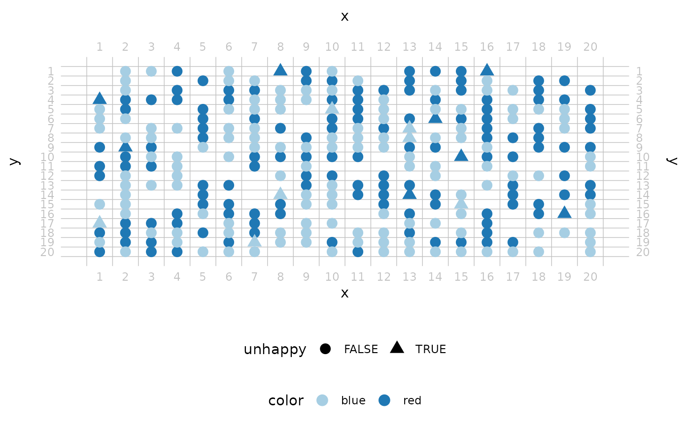
#> [1] "Tick 2 finished in 22.95 secs:"
#> [1] "  mean_similar: 0.562925170068027"
#> [1] "  share_unhappy: 0.00714285714285714"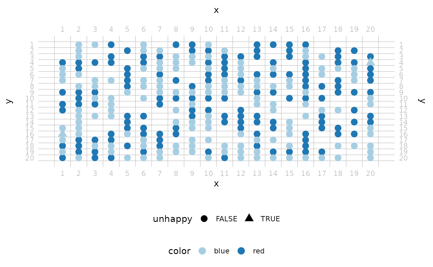
#> [1] "Tick 3 finished in 22.63 secs:"
#> [1] "  mean_similar: 0.56875"
#> [1] "  share_unhappy: 0.00357142857142857"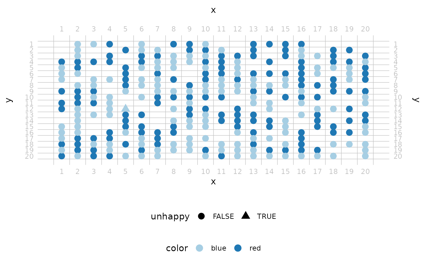
#> [1] "Tick 4 finished in 22.658 secs:"
#> [1] "  mean_similar: 0.572380952380952"
#> [1] "  share_unhappy: 0"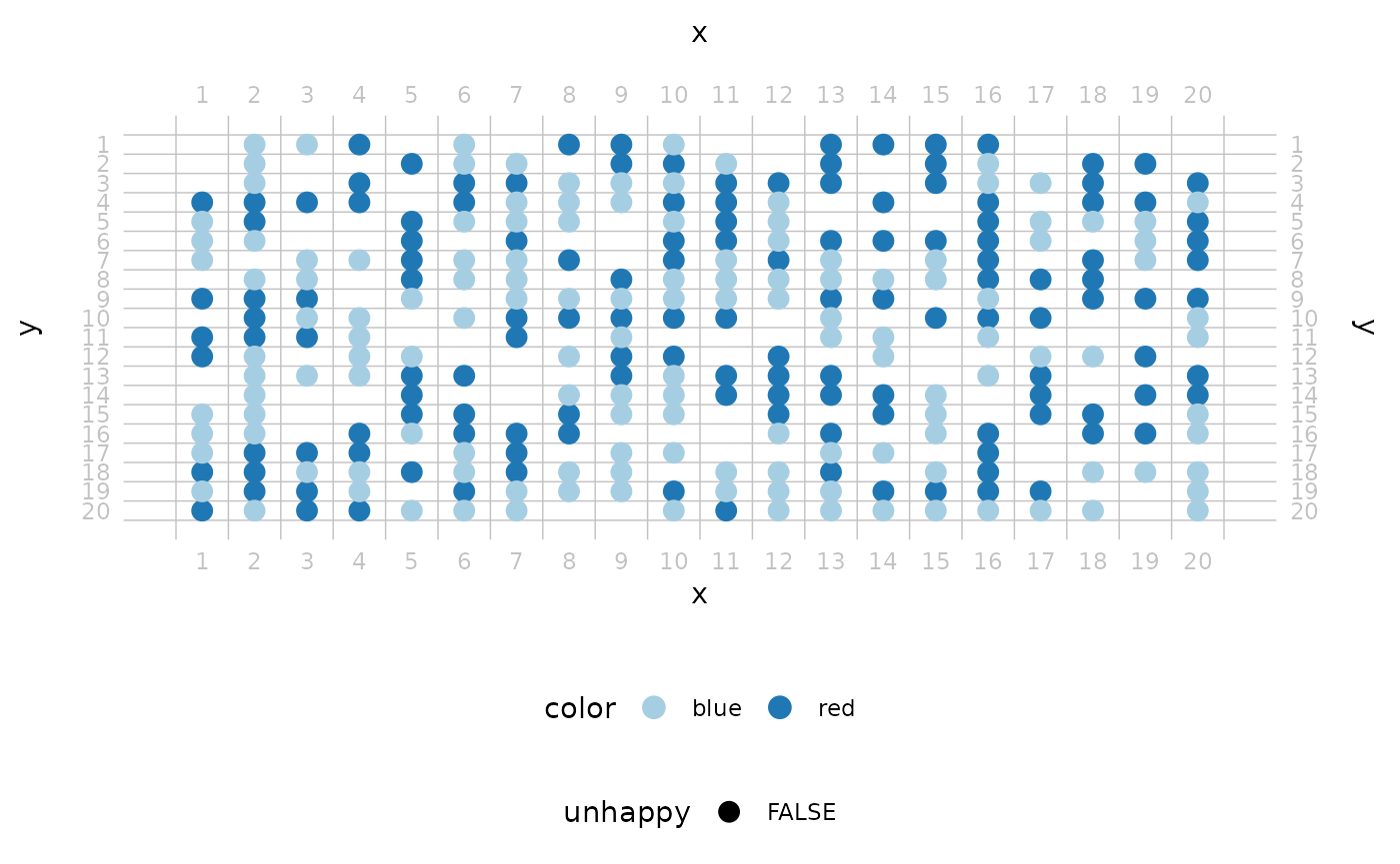
To manually inspect how everything went, we can just look at the environment or have it output all the agents.
e
#> # A tibble: 4 × 6
#>   .tick mean_similar share_unhappy .runtime      .n_agents_after_tick
#> * <dbl>        <dbl>         <dbl> <drtn>                       <int>
#> 1     1        0.499       0.0536  22.69281 secs                  280
#> 2     2        0.563       0.00714 22.95015 secs                  280
#> 3     3        0.569       0.00357 22.62952 secs                  280
#> 4     4        0.572       0       22.65765 secs                  280
#> # ℹ 1 more variable: .finished_after_tick <lgl>
#> # ABM grid environment
#> * 20x20, 280 agents
#> * 0 environment characteristic(s),
#> * 2 environment variable(s),
#> * 1 environment rule(s),
#> * ended after 4 ticks

e %>%
  convert_agents_to_tibble()
#> # A tibble: 280 × 6
#>    .id   color    .x    .y similar unhappy
#>    <chr> <chr> <int> <int>   <dbl> <lgl>
#>  1 A1    red       7    17   0.571 FALSE
#>  2 A2    red      17    13   0.25  FALSE
#>  3 A3    red       7    16   0.833 FALSE
#>  4 A4    red       6    19   0.286 FALSE
#>  5 A5    red      20     6   0.4   FALSE
#>  6 A6    red      14     9   0.333 FALSE
#>  7 A7    red       8    15   0.4   FALSE
#>  8 A8    red      19    16   0.5   FALSE
#>  9 A9    red      16    18   0.8   FALSE
#> 10 A10   red      13    16   0.4   FALSE
#> # ℹ 270 more rows
Ultimately, we are interested in how average similarity and the share of unhappy agents went down:
e %>%
  ggplot(aes(x = .tick,
             y = 100*share_unhappy)) +
  geom_line() +
  scale_x_continuous('Time [ticks]') +
  scale_y_continuous('Share of unhappy agents [%]') +
  theme_minimal() +
  ggtitle('Unhappiness over Time')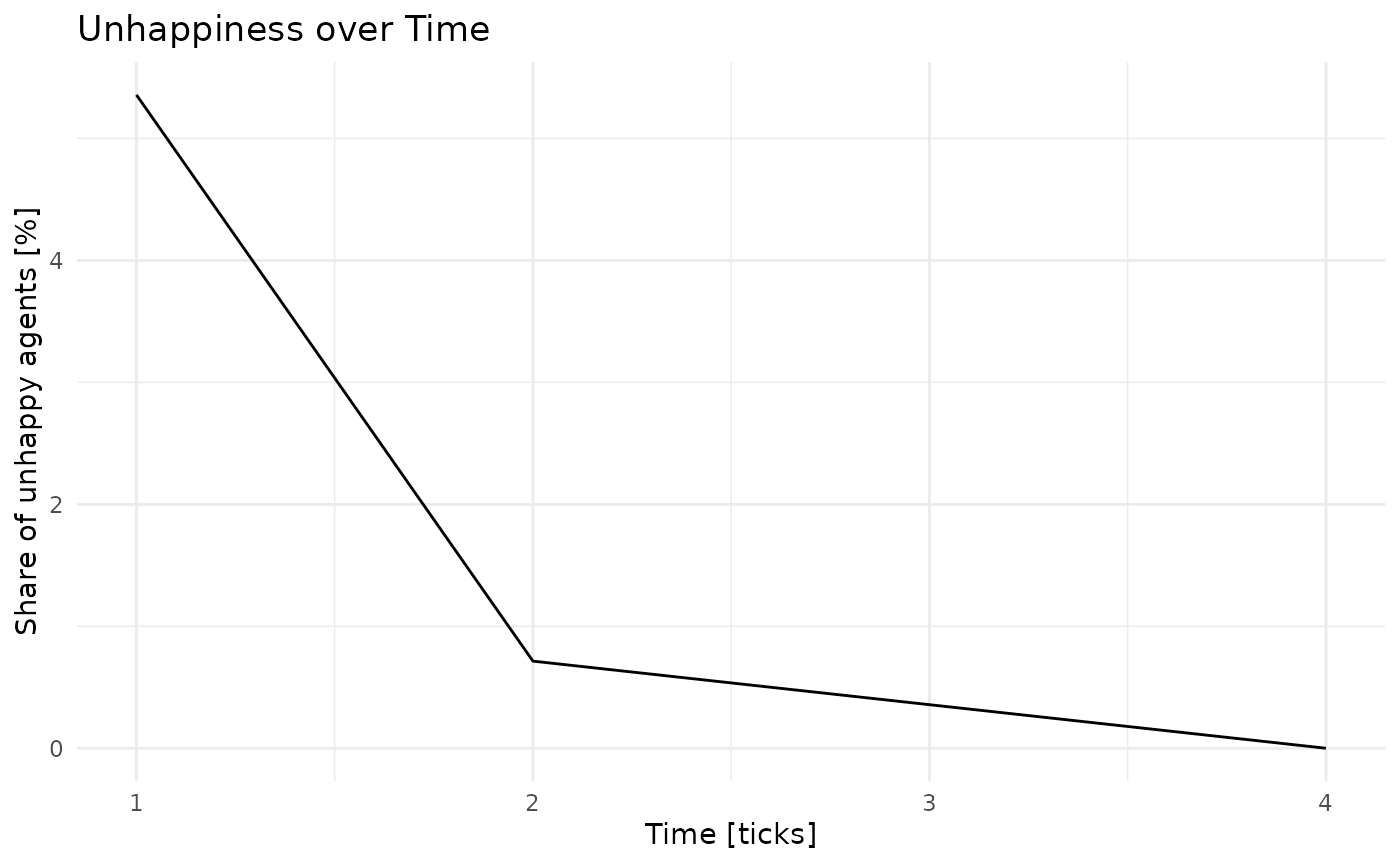
e %>%
  ggplot(aes(x = .tick,
             y = 100*mean_similar)) +
  geom_line() +
  scale_x_continuous('Time [ticks]') +
  scale_y_continuous('Average share of similar agents in neighborhood [%]') +
  theme_minimal() +
  ggtitle('Mean Similarity over Time')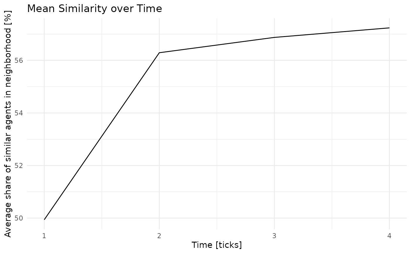
We can compile relevant data for any publication we’re preparing through the ODD protocol:
e %>%
  odd()
#> # A tibble: 7 × 4
#>   `ODD category`  Element                          Content `tidyABM information`
#>   <chr>           <chr>                            <chr>   <chr>
#> 1 Overview        Purpose and patterns             "Brief… NA
#> 2 Overview        Entities, state variables, and … "List … ABM grid environment…
#> 3 Overview        Process overview and scheduling  "Provi… environment rules: s…
#> 4 Design concepts Design concepts                  "This … see the iteration in…
#> 5 Details         Initialization                   "Speci… See the list of agen…
#> 6 Details         Input data                       "Repor… NA
#> 7 Details         Submodels                        "Repea… NA